Tuesday, June 15, 2021

Chapter 2: How to I start programming?

There are many programming language out there but we will only focus on Python as it is easy to learn and follow.


For Parents

You will need to setup the computer for your child by installing Python. Below are 2 videos which shows how you can install Python and Jupyter Notebook on your Computer. 


In case you missed it, to start Jupyter Notebook, you need to start the server by the command "jupyter notebook" in Command Prompt (CMD). Once you startup Jupyter Notebook, create your first  notebook by clicking on "new"->"Python 3"


As usual the first attempt at programming is the "Hello World" program and it can be done by the code:

print("Hello World")

To execute this code, press the "Run" button or "Ctrl"+"Enter". You will see the printout below.


For Children
Now that your parents has done up the setup, it is time to have some fun with programming. 
Try to print some other stuff such as:

print("Once, there was a boy who became bored when he watched over the village sheep grazing on the hillside.")
print("To entertain himself, he sang out, “Wolf! Wolf! The wolf is chasing the sheep!”")


This "print" function allows the computer to printout a text. Have you notice some other characteristics of the "print" function? 
- each print will output exactly one line
- the text that goes into the print is the "Input" of the program.
- the text that got printed is the "Output" of the program. 
- the text does not change, it is the same text each time you Run the program

You must be wondering, how then can I make the text change in different Run?
The function "input" will help address this. Try the below and the program will ask you to enter a value.

In this case, the function "input" also returns a value and it is stored in the variable, val.

val = input("Enter a input")

This val will then have the value you entered and can be printed using:

print(val)


Do note that the values between the quote "" are known as Strings. This is 1 of the datatype we commonly use in Python. We also have Integers (1,2,3,4,...) , Float (e.g. 1.1, 3.5, 4.666666).

Have fun till the next chapter!


Saturday, April 3, 2021

Chapter 1: Introduction to Computer Programming

We uses computer everyday and they come in different shape and sizes. The following video introduces what a computer do.


After watching the above video, can you name a few devices that is also a computer?


Typical computers has input and output. 

Input are data/information provided to a computer, typically they are 

    - Keyboard


- Mouse


After reading the input provided, the computer generate Output, typically they are shown in 

    - Display


But there are also other smaller computers, can you name the input and output of the following devices:

1) Mobile devices such as iPad, mobile phones

2) Washing Machine

3) TV


Did you notice that with input, the computer is smart enough to generate a corresponding output? Programming allows a computer to generate these input and this course will teach you how they are generated.

Thursday, September 12, 2019

Quick help on Writing C Extension for Python

Here are a few links to the website which I think is helpful in doing this:

The below 3 link will help you understand the basic of building from window:

https://docs.python.org/3/extending/extending.html
https://docs.python.org/3/c-api/module.html#c.PyModuleDef
https://stackabuse.com/enhancing-python-with-custom-c-extensions/
https://stackoverflow.com/questions/49299905/error-lnk2001-unresolved-external-symbol-pyinit
https://docs.python.org/3/c-api/structures.html

After which, the challenge is to compile/link it to the Python project. The challenge I have is when compiling the code, you cannot just use a typical compiler from the IDE. Rather I found out that you have to use the relevant command prompt:
https://docs.python.org/3/extending/windows.html
https://docs.microsoft.com/en-us/cpp/build/how-to-enable-a-64-bit-visual-cpp-toolset-on-the-command-line?view=vs-2019

For example:

cl /LD /I <Path to Python36/inclulde> spammodule1.c <path to python36.lib>
e.g.
cl /LD /I C:\Users\username\AppData\Local\Programs\Python\Python36\include\  spammodule1.c C:\Users\username\AppData\Local\Programs\Python\Python36\libs\python36.lib


At this point, I got stucked because I am not able to proceed to how to use the DLL and LIB files.

However, I found out that you can also use the distutils method to compile into .py files:
https://docs.python.org/3/extending/building.html

For example:
<Python.exe path> setup.py build
C:\Users\username\AppData\Local\Programs\Python\Python36\python.exe setup.py build

I find this method easier as it will do compilation as well as typical installation that allow you to use it like any other Python Module. Do note however that you need to include the path into the Python Interface:

https://stackoverflow.com/questions/28326362/pycharm-and-pythonpath


Saturday, August 24, 2019

Analysing Turf Club Data - Age does matter

In the past few weeks, I have been exploring data science and having read about Bill Benter I decided to also explore Data published on Turf Club. I managed to scrape the Singapore Turf Club and pull ut the following data:

Horse Performance
Jockey Performance
Race information

The pulling of information was relatively easy but I spend a lot of time cleaning up the data. The following are some record of what I found.

Horse Age
My initial thoughts were that horse age would matter since intuitively, the older any organism gets, the less likely it will be as strong. But it turn out that horse age does not matter. This means a old horse may still win a younger ones. This may make sense because I imagine myself to be a horse owner and I would also want to optimize the capability of my horse. This means I will not take part in competition that I have no chance of winning.


Jockey
I notice that for some horses, the same Jockey gets to ride them while other horses, the Jockey keeps changing. Some jockey has higher winning percentage while others are lower than average.

Age - Hypothesis 1
Horse age has an impact to winning.
I do not see a significant change in distribution for winners vs losers vs all population. If anything it shows that owners are less likely to send old horses for competition.


Even for old horses, the winning (1st or 2nd) rate is about 14% and that is just 1+% off the fair winning rate of 16+% (1/12*2). So it is fair to say every horse has an equal winning rate.

The best way of doing this is of course to conduct an hypothesis test but I did not go any further since I also believe surface information will not get me any extra information.


First time riding - Hypothesis 2

In this hypothesis, I think it matter if the jockey is riding the horse the first time. He may not have established a good understanding of the horse and this may affect the chance. So here we did some analysis:

Overall Analysis:

My finding is that young horses react very well to new ridership. Total probability of any horse winning (1st or 2nd) for all age is generally high at 25%:


Specifically, for age less than 1500 years is higher at 30%:


For older horses, there is no advantage in terms of probability:

Nth riding - Hypothesis 3
What about riding after once or twice or Nth time? Many a times I realized a horse is being rode by the same Jockey for an extended period of time. Is there an advantage to using the same Jockey?

It is found that older horses generally do not perform well to repeatedly being rode by the same Jockey:


Saturday, May 26, 2018

How to use Python in Excel

Here is a simple way to use Python in Excel which most would like since Python is a very quick and easy way to get things done.

Pre-requisite:

MS Excel
Excel Python
Windows extension for python

There are many tutorial which guides you to how this can be done. Please refer to the link in the reference.

After installation, you may encounter a bunch of issues, please refer to the troubleshooting page, I managed resolve everything from information found in this page.

You will see the Excel Python Tab available in Excel:


There are only 2 buttons:

1) Setup ExcelPython: Gets you started by creating a Python file and link it to your current workbook
2) Import Python UDF: Extract Python functions you created to Excel so you can use them directly without writing any VBA.

Click the first button to setup things. You will find a <worksheetfilename>.py file created in the same folder. What you have to do is to code functions in that Python file. E.g.

Workbook name: //path/Book1.xlsm
Associated Python file: //path/Book1.py

Next,click on the 2nd button to import the functions you have written and you are done!
Now you just need to use the same function name to execute your python functions.

Please find the attached example here.

Reference:
https://github.com/ericremoreynolds/excelpython/blob/master/docs/tutorials/Addin01.md

Friday, May 26, 2017

FE Trivial Part 1 - Relationship between Caplet and Option on Zero Coupon Bond

Caplet Payoff:

$X_{t_i}= N.\tau_i.Max(0,L(t_{i-1},t_i)-K)$

Given that forward rate:

$\tau_i.L(T_{i-1},T_i) = \frac{1-P(T_{i-1},T_i)}{P(T_{i-1},T_i)}$

Caplet Payoff:
$X_{t_i}$
$= N.\tau_i.Max(0,L(T_{i-1},T_i)-K)$
$=N.Max(0,\tau_i.L(T_{i-1},T_i)-K.\tau_i)$
$=N.Max(0,\frac{1-P(T_{i-1},T_i)}{P(T_{i-1},T_i)}-K.\tau_i)$

Discounting to today:
Caplet Price:
$= P(T_{i-1},T_i).N.Max(0,\frac{1-P(T_{i-1},T_i)}{P(T_{i-1},T_i)}-K.\tau_i)$
$= N.Max(0,1-(P(T_{i-1},T_i))(1+K.\tau_i))$
$= (1+K.\tau_i).N.Max(0,\frac{1}{(1+K.\tau_i)} - P(T_{i-1},T_i))$
$= N_{zero}.Max(0,K_{zero} -S_{zero})$

This the pricing of a put option on a Zero Coupon Bond with

Notional: $= (1+K.\tau_i).N$
Strike:$=\frac{1}{(1+K.\tau_i)}$

This will be important when we compare with Hull White 1 Factor Zero Coupon Bond Put European Option. Under the Hull White 1 Factor model, the close form solution is:

$Put_{zero} (t_0,t_1,t_2,K_{zero}) = K_{zero}P(t_0,t_1)\phi(-h+\sigma_{zero})-P(t_0,t_2)\phi(-h)$

Where
$\sigma_{zero}= \sigma_{black}\sqrt{\frac{1-e^{-2a(t_1-t_0)}}{2a}}B(t_1,t_2)$
$h=\frac{1}{\sigma_{zero}}ln{\frac{P(t-0,t_2)}{P(t_0,t_2)K_{zero}}+\frac{\sigma_{zero}}{2}}$

source


Wednesday, February 22, 2017

xVA


This article is to document what I have learned about XVA. I will first layout a few idea and continue to improve this as I find out more. Source of these information are from books such as

1 ) The XVA Challenge
...

For an introduction, the point of calculating XVA is to find out the various cost of transaction in banks, from inception to maturity. Various stakeholders are involved in this process:

1) Dealers
a. Traders
There are different kind of traders in a bank, some are just doing flow business, others are doing proprietary trading. Typically, the head of desk will treat the desk trading business as any other business. He/She will consider the cost of operating this desk. XVA will form part of the operation cost.
b. Structurers
The trades done by structures are huge chunky trades as compared to traders. These are typically longer term as well. The counterparties involved are typically entities such as fund house, security firms and corporates. These counterparties have significant credit risk compared to interbanks trades. Therefore, XVA will form an important cost to the desk.

2) CVA Desk
This desk is responsible for hedging the CVA (one part of XVA) which is directly linked to the credit risk of counterparties. Hedges are typically done using CDS or proxy trades which is correlated to counterparties. Traders and Structurer will pay CVA cost to this desk and as such the credit risk associated with the trade is taken to be hedged out with this desk. This desk will be interested in the CVA Greeks as they are required to managed the CVA according to the movement in the market.

3) Risk Managers
This function is involved in computing, monitoring and reporting the exposure of the bank to management and regulators.


XVA Components

CVA
Simpliest among these, just go Google

DVA
The flip side of CVA.

FVA


KVA

For every trade done in bank, there is a capital charge associate with it. These charges are amount which banks are required to set aside for mitigating counterparty credit risk. In the past, banks ignore this cost and uses quick and dirty way such as using minimum charges to transactions. Today, banks have became more sophisticated and implements KVA is to properly price the cost of setting aside such Capital for regulatory purposes.

3 factors to Capital Requirement for OTC Derivatives
- Default risk capital charge
Potential default charge of counterparty i.e. CCR

- CVA capital Charge
CVA sensitivity due to movement in Credit Spread

- Market Risk Capital Charge (insignificant since regulator has implement rule to reduce this)
These are capital charges arises from doing hedges.

- Capital Charge on exposure to CCP is very little.

Formula
KVA  =-$\sum_{i=1}^{m} $EC(t_i)xCC(t_i)X(t_i-t_(i-1))XS(t_i)

Margin Valuation Adjustment (MVA)
As the name suggest, this adjustment is related to margin associated with trades. Margin are charged to protect against default, so it is expensive and not re-hypothecated; it is regarded as a separate amount.

It consist of:
1) Initial Margin (and other financial resources required by Central Counterparty (CCP)
When a bank (Clearing Member) deal with counterparty via CCP, they are required to post an Initial Margin (IM) so that if they default, this margin can help buffer against the lost suffered by CCP.
These are cost to banks as the interest paid by CCP are less than the funding cost required.

Questions:
What benchmark is used by CCP to pay clearing members for IM?

2) Bilateral IM
This is required when both parties are required to post initial margin to each other.

3) Contingent IM

How are IM calculated?
IM calculation are determined by using VAR or expected shortfall. This means they need to specify % confidence interval and time horizon.

MVA  =-$\sum_{i=1}^{m} $EIM(t_i)x(FC(t_i)-S_im)X(t_i-t_(i-1))XS(t_i)

Where $EIM = discounted expected IM, $FC is funding cost and $S_IM is the remuneration from posting IM.

EIM are calculated using simulation over 99% confidence interval with 10 days horizon.

Comparison with FCA
- MVA is the funding cost associated with worst-case movement of portfolio during a 10 day horizon. This is due to the fact that the trade is collateralized and the 10 days is to cover the situation where there is a default discovered only after 10 days, by which the market would have moved.

-FCA is the funding requirement over the life of the trade.

Questions:
What is the flow of calculating MVA?


XVA consists of a few components summarized in the table below:

ColVA
CVA
DVA
FVA
KVA
MVA
Uncollateralised
One-way collateralised
()
()
Traditional two-way collateralised
()
()
Single-currency two-way collateralised
()
()
()
Collateralised with bilateral initial margin
()
()
Centrally cleared (direct)
()
()
Centrally cleared (indirect)
()
()
Obtained from the book: The XVA Challenge


Sunday, May 29, 2016

Using C# in Excel Part I


In the typical work environment, it is very common for non-programmer to try to use VBA to create process automation. And it is no doubt a fast way to implement automation with the least computing knowledge. However, when the complexity is high and coupled with high volume, this will significantly slow down the PC and creates bad user experience. Especially when we are doing it for another user, we might wonder if there is a better solution?

In this post, I explore how I can use C# to code automation functions and to implement it onto VBA. This is nothing new so all the information required was obtained from other experts online. Specifically, I got most of the information here.

Step 1:
Using Visual Studio Community 2015, create a class library:


Step 2:
Communication with VBA require the code to be in "COM Library", so to do this
a)  You have to check "Make Assembly COM-Visible" checkbox under 
Project -> Properties -> Assembly Information


b) Next, we will need to register it so that VBA will be able to recognize this when we start coding in VBA. But you also won't want to register all the library you developed on the developing machine as it will make your PC very messy. So I will come back to this setting again later to explain how to remove it. 

Under the same property window, go to the build tab, Project -> Properties -> Build.
Check the ‘Register for COM interop’ checkbox.


Step 3:
The setup is completed and you can start writing your code. The following is a simple code to output a string:

using System;
using System.Collections.Generic;
using System.Text;
 
namespace DotNetLibrary
{
    public class DotNetClass
    {
        public string DotNetMethod(string input)
        {
            return "Hello " + input;
        }
    }
}

Step 4:
Compile and start using in VBA! For example, we now try to use Excel to call the above method.
In Excel, enter the VBA programming window by pressing ALT+F11. You will find that library you created under Tools -> Reference. In this case, the library is called blog.


To access the DotNetMethod, you can invoke by using the following VBA Code:

 
Sub test()
    Dim clest As New DotNetClass
    Dim test As Variant  
    MsgBox (clest.DotNetMethod("ABC"))
 
End Sub

Run the macro ("F5") and you will see the msgbox:


Step 5:
Up till now, what you have seen how to get to use functions in VBA in your own PC. But suppose you want to develop it on your own PC and implement it onto another PC, how can you do it?
So starting from Step 2b, we don't really need to check the "Register for COM Interop" because what we really need is just the DLL file. But now that we checked it, how can we remove it? This is simple, we just need to uncheck and compile your project again and it will be unregistered.

So once you unregistered, whatever you compile will not appear on VBA Reference. You will need to take the DLL and copy to the target PC and start the registration manually.

Register:
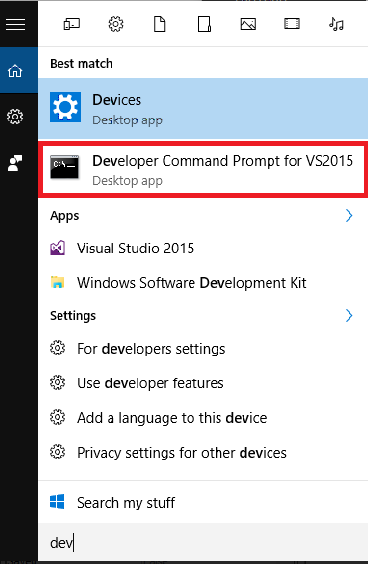
To register you will need to use "regasm" function from Visual Basic Command Prompt. You can easily access this by typing "Dev" after pressing the "Window" key:


Navigate to your project directory containing the DLL file and now you are ready to use the "regasm" function (assuming the name of your dll is "dllname"). Type the following to create the ".tlb" required for VBA to recognize your DLL file.

regasm /tlb  dllname.dll

After typing the above command, you will see that the library will appear in the same place mentioned in Step 4,


If you want to unregister, you can type the following command:

regasm /u dllname.dll

As you can see, all these registering are not very transparent to the developer on what exactly is happening. So there will be times where you are not able to unregistering. And when that happens, a quick way is to open your project and repeat what is mentioned at the beginning for Step 5, i.e. check option -> compile, uncheck option -> compile. This will let Visual Studio do the unregistering for you.


If you want a quick start, you can use the sample project here. Enjoy coding!


Saturday, September 26, 2015

Charting in R - Part I

The toughest step to doing things like quantitative analysis for trading and backtesting is to understand how to use the tools available in the market. The choices available are as follows:

  1. Excel
  2. R
  3. Python
  4.  C/C++

Excel allows you to see and manipulate data easily but you cannot see trend properly. For example, if you wish to chart data in Excel, this is what you will get:


This graph looks acceptable for simple presentation. But if you want to do analysis, you would want to be able to add a complex indicator easily. In Excel, you can only do that by manipulate all the data in excel and plot another graph on it. To do complex analysis of data it will be much better to do it with scripting API available in the market. If you know your stuff, you can do things pretty fast. But it takes a hell lot of effort to even get started. To illustrate the advantage of using API, the following is created using GOOGLE prices and R.


As someone who had tried both Python and R, my opinion is that the later is a better tool to do charting. So I documented some tips to get you started on R.

What you need to install
R(Here you will find the latest version but I am using version 2.15)
Quantmod (To quickly install, follow instruction here to download and install all that you need)

Once you are done, you can quickly load data with the following sample code (modified from code taken from here) and data.

Code:

library(quantmod)
require (zoo)
dataFile_strip2 <- "testinput.csv"
dataDir <- "C:/Users/Ken/Documents/R/CSV Data"
file2 <- paste(dataDir,"/",dataFile_strip2,sep="")
zz <- read.zoo(file2,header = TRUE,sep=",",index.column=1, format = "%d/%m/%Y %H:%M")
xx<- as.xts(zz)
chartSeries(xx)


testinput.csv:
DateTime,Close,High,Low,Open,Volume
12/08/2015 21:30:00,112.53,112.61,112.5,112.5,877727

Other Reference:
https://cran.r-project.org/web/packages/zoo/vignettes/zoo-read.pdf

Friday, April 3, 2015

Using C++ and VBA in Excel - Part II

One way of doing this is as stated in my previous post. But many beginner in C++ would be daunted by the amount of basics in Computing required to understand why it work. To simplify this process, we can use XLW to implement wrapper easily. The only requirement is to know basic C++ and a simple 3 step process.

Step 1
First, you will need Microsoft Visual Studio and install XLW onto your PC. Use Template Extractor:


Choose the Visual Studio version correctly. Note that if you are using Visual Studio 2012 you will need to choose VC10 instead of VC12.

Step 2
The template you just created is a skeleton VS project which allow you to develop XLL. Once you fire up template.sln, you will notice that the project is setup nicely for you to start development.

As an example, I did a test function that return the square of a number:


As usual, for every function you create in C++ you will need to declare it in the header. But this time, you will need to declare it onto cppinterface.h. This is the most important step you need to do in C++ and you are ready to compile the project.

Step 3
The compilation will create the XLL file and you will be able to find it in the output folder. In this case, I am using debug mode and "Template.xll" will therefore appear in the debug folder. Launch "Template.xll" and you should not encounter any error, if so then there must be an error in the compilation process. If there are no error then you can create a new worksheet and start using the "helloworld" function you just created.


Tuesday, October 7, 2014

Executing an executable from VBA

For people in the software industries such as consultants, developers and even managers, they will very often need to handle different versions of software. Many a times, these versions are stored in different places. This means we will need to memorize these directories and every time we need to access them, we will need to navigate to these directories. The best way to overcome these is to tabulate the versions in Excel. But it is insufficient as it we are not able to start the software from the tables in excel natively.

By using VBA you can do this with the "Shell" command. The problem is with this is that you can only execute files that has no dependency on the folder you are executing it from. This means the environment paths and parameters needs to be setup correctly in Windows.

To overcome this limitation, I combined what I posted previously to build a table having the ability to execute a software from Excel. Instead of building your own DLL, what you need is to use the existing DLL (Refer to here for more details on how this is done in VBA):

Public Declare Function ShellExecute Lib "Shell32.dll" Alias "ShellExecuteA" _
  (ByVal hwnd As Long, _
   ByVal lpOperation As String, _
   ByVal lpFile As String, _
   ByVal lpParameters As String, _
   ByVal lpDirectory As String, _
   ByVal nShowCmd As Long) As Long

By declaring this you are effectively using the "ShellExecute" library from Shell32.dll to execute lpFile from lpDirectory.This will allow user to have more flexibility in building UI that will execute files upon clicking in VBA. An example of using the above is as follows:


RetVal = ShellExecute(0, "open", "C:\folder\client.cmd", "<arguments>", _
                        "C:\folder\", SW_SHOWMAXIMIZED)

Saturday, April 26, 2014

SABR Model - Introduction

The famous option pricing Black-Scholes framework assumes that the asset price follows the stochastic process:

$dS_{t} = rd_t+{\sigma}dw_t$
where $w_t$ is a Brownian motion and $r$ is the risk free rate.

This simply means the dynamics of asset price is a random variable following a lognormal distribution with constant volatility of ${\sigma}$. This evaluates to the option pricing formula:

$C({\sigma}, r, S_t, K) = S_t{N(d_1)} - KN(d_2)$
where $d_1 = \frac{(ln(\frac{S_t}{K})+\frac{1}{2}(r+\sigma^2)t}{\sigma\sqrt{t}}$ and $d_2 = d_1-\sigma\sqrt{t}$

However, in practice, the option price implied by the market indicates that there is different volatility for different strikes. Furthermore, stock prices has distribution with fat tail and has higher peak relative to Normal distribution. This implies that there is a mixture in distributions with different variances. This is the motivation for developing volatility models such as Local Volatility, Heston Model, SABR Model and etc. In this post, the SABR model will be introduced briefly. The SABR model is a stochastic volatility model developed by Patrick Hagan et al. It has the following dynamics:

$dF_t = F_t^{\beta} {\sigma}_t dW_t$ , $0≤{\beta}≤1$
$d{\sigma}_t = v{\sigma}_t dB_t$ , $v>0$
$d{<}W,B{>}_t = {\rho}dt$ , ${\rho}ϵ[-1,1]$
${\sigma}_0 = {\alpha} >0$

$where$
${\beta}$ : Describes the forward rate model.
$v$ : Lognormal volatility of volatility
${\rho}$ : Correlation between Forward rate and Volatility
${\alpha}$ : ATM volatility

This dynamic is clearly different from the Black Scholes framework and the market is quoted in Black's volatility for instruments such as cap/floor, swaptions and etc. What Hagan et al. did was to use this dynamics to price a European option. In the process of this evaluation, it is found that with some estimation techniques, the pricing using SABR dynamics is close to the normal model. From the normal model, it is then further derived that the pricing using SABR will approximate to Black's lognormal model.

The formula for the implied Black's volatility is as follows:

${\sigma}_{implied} (K,f)=\frac{\alpha}{((fK)^(\frac{(1-{\beta})}{2}) (1+\frac{(1-{\beta})^2}{24} log^2(\frac{f}{K})+\frac{(1-{\beta})^4}{1920} log^4((f/K)+⋯ ) ) )} \frac{z}{X(z)})$
$(1+\frac{(1-{\beta})^2}{24} \frac{{\alpha}^2}{(fK)^(1-{\beta})} + \frac{1}{4} \frac{{\alpha}{\beta}v{\rho}}{(fK)^\frac{1-{\beta}}{2}} +\frac{2-3{\rho}^2 }{24} v^2 ) t_ex+⋯)$
$where$
$z=\frac{v}{{\alpha}} (fK)^(\frac{1-{\beta}}{2})log(\frac{f}{K})$
$X(z)=log(\frac{\sqrt{1-2{\rho}z+z^2 }+z-{\rho})}{(1-{\rho})})$
This series of proving shows that Black's volatility quoted in the market can be modeled with SABR model. All that needs to be done is to calibrate the SABR parameters such that the volatility matches market quotes.

Saturday, December 28, 2013

Natural Cubic Spline interpolation (Application)

It has been a long journey from Theory to Derivation and now we are onto application. With all the theories and equations we obtained, we will now apply them and conduct interpolation.
For (n+1) points we now have 3 generic equations
$\frac{3(y_{i+2}-y_{i+1})}{(x_{i+2}-x_{i+1})^2} +\frac{3(y_{i+1}-y_i)}{(x_{i+1}-x_i)^2} = \frac{k_i}{x_{i+1}-x_i }+k_{i+1}[\frac{2}{x_{i+1}-x_i} +\frac{2}{x_{i+2}-x_{i+1}}]+\frac{k_{i+2}}{x_{i+2}-x_{i+1}}$           —(1)
$3\frac{y_{n+1}-y_n}{(x_{n+1}-x_n)^2}= \frac{2k_{n+1}}{x_{n+1}-x_n}+ \frac{k_n}{(x_{n+1}-x_n)}$ —(2)
$3\frac{y_1-y_0}{(x_1-x_0)^2} = \frac{2k_0}{x_1-x_0}+\frac{k_1}{x_1-x_0}$  —(3)
For i=[0,n-2]

The unknow here is k which is $f_i'(x_i)=c_i$, we have also seen that the rest of $a_i,b_i, d_i$ are all known as follows:
$a_i=\frac{1}{3}[\frac{(k_{i+1}-k_i)}{(x_{i+1}-x_i)^2}-\frac{2b_i}{(x_{i+1}-x_i )}]$ ---(4)
$b_i= \frac{3(y_{i+1}-y_i )}{(x_{i+1}-x_i)^2} - \frac{k_{i+1}+2k_i}{(x_{i+1}-x_i)}$    ---(5)
$c_i=k_i$    ---(6)
$d_i = y_i$    ---(7)

What is left now is to find k and it can be found by applying equation (1) - (3) and put them into matrix form and solve k using simple linear algebra.

$Wk = F$
$k_{(n+1)x1}=[k_0,k_1,...,k_n]^T$
$F_{(n+1)x1} =[ f_0,f_1,...,f_n]^T$
Where $f_i$ are the Left Hand sides of (1)-(3) and W is the (n+1)x(n+1) matrix formed by the Right Hand side of (1)-(3).

By obtaining the inverse of W,

$k = W^{-1} F$

we can solve for k.

To do interpolation for a value x, follow the following algorithm:

Step 1:
Find the interval $[x_i,x_{i+1}]$ by which x belongs.

Step 2:
Apply (4)-(7) to obtain the cubic equation coefficient.

Step 3:
Plug in the coefficients into the equation:
$y(x) = a_i(x-x_i)^3 + b_i(x-x_i)^2+c_i(x-x_i)+d_i$

Done! Now you got an estimated value of y(x)!

Tuesday, December 24, 2013

Natural Cubic Spline interpolation (Derivation)

Recap that in our previous post, we introduce how cubic spline interpolation can be applied to a n+1 points to produce a smooth curve. There will be a total of n curves each described by:
$f_i (x) = a_i(x-x_i)^3 + b_i(x-x_i)^2 + c_i (x-x_i) + d_i$

The conditions for a natural cubic spline is given by the following:

$f_i (x_i) = a_i(x-x_i)^3 + b_i(x-x_i)^2 + c_i (x-x_i)+d_i = y_i$    (1)
$f_i (x_i) = f_{i+1}(x_i)$                                                                         (2)
$f_i '(x_i) = f_{i+1}'(x_i)=c_i$                                                                (3)
$f_i ''(x_{i+1}) = f_{i+1}''(x_{i+1})=2b_i$                                                      (4)
$f_0''(x_0) = 0$                                                                                   (5)
$f_{n-1}''(x_{n-1}) = 0$                                                                            (6)

From here we will derive the solution to conduct cubic spline interpolation. The end results will be as specified in Wikipedia. The idea is the same as when you try to solve simultaneous equations and place them into systems of linear equations and solve them using simple linear algebra.

From (3) we are going to express everything in $f_i '(x_i) = f_{i+1} '(x_i) = k_{i+1}$. 
First we obtain $a_i$ in terms of $b_i$ and $k_i$

$f_{i+1}'(x_i)=c_i$     
$c_{i+1}-c_i= 3a_i (x_(i+1)-x_i )^2+2b_i (x_(i+1)-x_i )$ 
$a_i=\frac{1}{3}[\frac{(k_{i+1}-k_i)}{(x_{i+1}-x_i)^2}-\frac{2b_i}{(x_{i+1}-x_i )}]$ (7)

From (4) we will get,
$f_{i+1}''(x_{i+1})=2b_{i+1}=6a_i(x_{i+1}-x_i)+2b_i$
$b_{i+1}-b_i= 3a_i (x_{i+1}-x_i )$                                                                             (8)

Next we will substitute (7) into (8) 
$b_{i+1}-b_i= 3*\frac{1}{3}[ \frac{k_(i+1)-k_i}{(x_{i+1}-x_i)^2} - \frac{2b_i}{(x_{i+1}-x_i )}]*(x_{i+1}-x_i ) $
$b_{i+1}-b_i= \frac{(k_{i+1}-k_i)}{(x_{i+1}-x_i )}-2b_i $
$b_{i+1}+b_i= \frac{(k_{i+1}-k_i)}{(x_{i+1}-x_i )}$                                                                    — (9)

Equation (9) will be used in one of the final substitution so let's just hang on to equation (9) first and we will come back to this later. Now we try to substitute (1) and (7) into (2) to express $b_i$ in terms of $k_i$:

$y_{i+1}= a_i (x_{i+1}-x_i )^3+b_i (x_{i+1}-x_i)^2+c_i (x_{i+1}-x_i )+d_i$

$y_{i+1}-y_i= \frac{1}{3}[ \frac{(k_{i+1}-k_i)}{(x_{i+1}-x_i)^2} -\frac{2b_i}{(x_{i+1}-x_i )}](x_{i+1}-x_i )^3+b_i (x_{i+1}-x_i)^2+k_i (x_{i+1}-x_i )$

$\frac{(y_{i+1}-y_i)}{(x_{i+1}-x_i)^2} = \frac{1}{3}[\frac{(k_{i+1}-k_i)}{(x_{i+1}-x_i}-2b_i ]+b_i+\frac{k_i}{(x_{i+1}-x_i )}$

$\frac{3(y_{i+1}-y_i )}{(x_{i+1}-x_i)^2} = [\frac{(k_{i+1}-k_i)}{(x_{i+1}-x_i)}-2b_i ]+3b_i+\frac{3k_i}{x_{i+1}-x_i } $

$b_i= \frac{3(y_{i+1}-y_i )}{(x_{i+1}-x_i)^2} -  \frac{(k_{i+1}-k_i)}{x_{i+1}-x_i}-\frac{3k_i}{(x_{i+1}-x_i )}$
$b_i= \frac{3(y_{i+1}-y_i )}{(x_{i+1}-x_i)^2} - \frac{k_{i+1}+2k_i}{(x_{i+1}-x_i)}$  —(10)

Finally substitute (10) into (9) to get a equation with only ks, ys and xs.
$\frac{3(y_{i+2}-y_{i+1} )}{(x_{i+2}-x_{i+1})^2} -  \frac{(k_{i+2}+2k_{i+1})}{(x_{i+2}-x_{i+1})}+\frac{3(y_{i+1}-y_i )}{(x_{i+1}-x_i)^2} - \frac{(k_{i+1}+2k_i)}{(x_{i+1}-x_i)}= \frac{k_{i+1}-k_i}{x_{i+1}-x_i}$

$\frac{3(y_{i+2}-y_{i+1})}{(x_{i+2}-x_{i+1})^2} +\frac{3(y_{i+1}-y_i )}{(x_{i+1}-x_i)^2} = \frac{k_{i+1}-k_i}{x_{i+1}-x_i}+ \frac{k_{i+2}+2k_{i+1}}{x_{i+2}-x_{i+1}}+ \frac{k_{i+1}+2k_i}{x_{i+1}-x_i}$

$\frac{3(y_{i+2}-y_{i+1})}{(x_{i+2}-x_{i+1})^2} +\frac{3(y_{i+1}-y_i}{(x_{i+1}-x_i)^2} = \frac{k_i}{x_{i+1}-x_i }+k_{i+1}[\frac{2}{x_{i+1}-x_i} +\frac{2}{x_{i+2}-x_{i+1}}]+\frac{k_{i+2}}{x_{i+2}-x_{i+1}}$ —(11)

With this equation we have exactly (n-1) such equations for i=[0,n-2] and we have (n+1) unknown. By using the 2 other equation (5) and (6), we will obtain the other 2 equations.

Therefore, subsitute i=n and (10 )into (4) 
$0= 6a_n (x_{n+1}-x_n )+2b_n$
$0= 2[\frac{(k_{n+1}-k_n)}{(x_{n+1}-x_n)^2} -\frac{2b_n}{x_{n+1}-x_n }](x_{n+1}-x_n )+2b_n$
$b_n   =\frac{k_{n+1}-k_n}{x_{n+1}-x_n }$
$3\frac{y_{n+1}-y_n }{(x_{n+1}-x_n)^2} = \frac{k_{n+1}-k_n}{x_{n+1}-x_n }+
\frac{k_{n+1}+2k_n}{x_{n+1}-x_n}$
$3\frac{y_{n+1}-y_n}{(x_{n+1}-x_n)^2}= \frac{2k_{n+1}}{x_{n+1}-x_n}+ \frac{k_n}{(x_{n+1}-x_n)}$ —(12)

Substitute i=0 into (10),
$b_0= \frac{3(y_1-y_0 )}{(x_1-x_0)^2} - \frac{k_1+2k_0}{(x_i-x_0)}=0$
$3\frac{y_1-y_0}{(x_1-x_0)^2} = \frac{k_1+2k_0}{x_1-x_0}$
$3\frac{y_1-y_0}{(x_1-x_0)^2} = \frac{2k_0}{x_1-x_0}+\frac{k_1}{x_1-x_0}$  —(13)


Equations 11-13 is the exact equations you will see in Wikipedia. Now the obvious question is "How are we going to use all these equations we derived to do Cubic Spline Interpolation?". This shall be reviewed in the upcoming post.